Make python fast with numba
Python is an interpreted language, so it's flexible and easy to use, but it can be slow. Learn how to make it 100 times faster by compiling it for your machine, with just one line of additional code. Notebook ready to run on the Google Colab platform

(c) Lison Bernet 2019
Introduction
"Python is an interpreted language, so it's way too slow."
I can't count how many times I heard that from die-hard C++ or Fortran users among fellow particle physicists!
True, python is an interpreted language and it is slow.
Even python advocates like me realize it, but we think that the (lack of) speed of python is not really an issue, e.g. because:
- The time spent computing is balanced by a much smaller development time;
- Some python tools like numpy are as fast as plain C;
- Profiling is easy, which means that one can find the parts of the code that are slow, optimize them, and even write them in faster languages so that they can be compiled and used from python.
What is less known is that python can also provide you with a direct access to your hardware for intensive calculations.
In this post, we will see how to translate python code into machine code for the CPU, to make it 100 times faster .
You will learn:
- a little bit about python decorators;
- what is numba , a just-in-time compiler that translates python code into fast machine code;
-
how to use
numba
to solve a few computing problems efficiently:
- the calculation of pi;
- finding the closest two points in a large dataset.
This is the first part of my series on accelerated computing with python:
- Part I : Make python fast with numba : accelerated python on the CPU
- Part II : Boost python with your GPU (numba+CUDA)
- Part III : Custom CUDA kernels with numba+CUDA (to be written)
- Part IV : Parallel processing with dask (to be written)
Running this tutorial
You can execute the code below in a jupyter notebook on the Google Colab platform by simply following this link .
Another possibility is to run the tutorial on your machine. For that, install anaconda if not already done, and then install numba, jupyter, and numpy with conda:
conda install numba jupyter numpy
Here is the notebook for this tutorial: numba_intro.ipynb . Start a jupyter notebook, and open this file to get started.
But you can also just keep reading through here if you prefer!
Python decorators 
With numba, the compilation of a python function is triggered by a decorator. If you already know what's a decorator, you can just skip to next section. Otherwise, please read on.
A python decorator is a function that takes another function as input, modifies it, and returns the modified function to the user.
I realize that this sentence sounds tricky, but it's not. We'll go over a few examples of decorators and everything will become clear!
Before we get started, it's important to realize that in python, everything is an object. Functions are objects, and classes are objects too. For instance, let's take this simple function:
def hello():
  print('Hello world')
hello
is a function object, so we can pass it to another function like this one:
def make_sure(func):
  def wrapper():
    while 1:
      res = input('are you sure you want to greet the world? [y/n]')
      if res=='n':
        return
      elif res=='y':
        func()
        return
  return wrapper
This is a decorator!
make_sure
takes an input function and returns a new function that wraps the input function.
Below, we decorate the function
hello
, and
whello
is the decorated function:
whello = make_sure(hello)
whello()
Of course, we can use the make_sure decorator on any function that has the same signature as
func
(can work without arguments, and no need to retrieve the output).
We know enough about decorators to use numba. still, just one word about the syntax. We can also decorate a function in this way:
@make_sure
def hello():
  print('Hello world')

hello()
There is really nothing mysterious about this, it's just a nice and easy syntax to decorate the function as soon as you write it.
just-in-time compilation with numba 
Numba is able to compile python code into bytecode optimized for your machine, with the help of LLVM. You don't really need to know what LLVM is to follow this tutorial, but here is a nice introduction to LLVM in case you're interested.
In this section, we will see how to do that.
Here is a function that can take a bit of time. This function takes a list of numbers, and returns the standard deviation of these numbers.
import math

def std(xs):
  # compute the mean
  mean = 0
  for x in xs:
    mean += x
  mean /= len(xs)
  # compute the variance
  ms = 0
  for x in xs:
     ms += (x-mean)**2
  variance = ms / len(xs)
  std = math.sqrt(variance)
  return std
As we can see in the code, we need to loop twice on the sample of numbers: first to compute the mean, and then to compute the variance, which is the square of the standard deviation.
Obviously, the more numbers in the sample, the more time the function will take to complete. Let's start with 10 million numbers, drawn from a Gaussian distribution of unit standard deviation:
import numpy as np
a = np.random.normal(0, 1, 10000000)
std(a)
The function takes a couple seconds to compute the standard deviation of the sample.
Now, let's import the njit decorator from numba, and decorate our std function to create a new function:
from numba import njit
c_std = njit(std)
c_std(a)
The performance improvement might not seem striking, maybe due to some overhead related with interpreting the code in the notebook. Also, please keep in mind that the first time the function is called, numba will need to compile the function, which takes a bit of time.
But we can quantify the improvement using the timeit magic function, first for the interpreted version of the std function, and then for the compiled version:
%timeit std(a)
%timeit c_std(a)
The compiled function is 100 times faster!
But obviously we did not have to go into such trouble to compute the standard deviation of our array. For that, we can simply use numpy:
a.std()
%timeit a.std()
We see that numba is even faster than numpy in this particular case, and we will see below that it is much more flexible.
Calculation of pi 
the number pi can be estimated with a very elegant Monte Carlo method.
Just consider a square of side L=2, centred on (0,0). In this square, we fit a circle of radius R=1, as shown in the figure below.
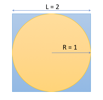
The ratio of the circle area to the square area is
$$r = \frac{A_c}{A_s} = \frac{\pi R^2}{L^2} = \pi / 4$$so
$$\pi = 4 r$$So if we can estimate this ratio, we can estimate pi!
And to estimate this ratio, we will simply shoot a large number of points in the square, following a uniform probability distribution. The fraction of the points falling in the circle is an estimator of r.
Obviously, the more points, the more precise this estimator will be, and the more decimals of pi can be computed.
Let's implement this method, and use it with an increasing number of points to see how the precision improves.
import random

def pi(npoints):
  n_in_circle = 0
  for i in range(npoints):
    x = random.random()
    y = random.random()
    if (x**2+y**2 < 1):
      n_in_circle += 1
  return 4*n_in_circle / npoints
npoints = [10, 100, 10000, int(10e6)]
for number in npoints:
  print(pi(number))
As you can see, even with N=10 million points, the precision is not great. More specifically, the relative uncertainty on pi can be calculated as
$$\delta = 1/ \sqrt{N}$$Here is how the uncertainty evolves with the number of points:
import math
# defining the uncertainty function
# with a lambda construct
uncertainty = lambda x: 1/math.sqrt(x)
for number in npoints:
  print('npoints', number, 'delta:', uncertainty(number))
Clearly, we'll need a lot of points. How fast is our code?
%timeit pi(10000000)
A few seconds for 10 million points. This algorithm is O(N), so if we want to use 1 billion points, it will take us between 5 and 10 minutes . We don't have that much time, so let's use numba!
@njit
def fast_pi(npoints):
  n_in_circle = 0
  for i in range(npoints):
    x = random.random()
    y = random.random()
    if (x**2+y**2 < 1):
      n_in_circle += 1
  return 4*n_in_circle / npoints
fast_pi( int(1e9) )
This took about 10 s, instead of 7 minutes!
A more involved example: Finding the closest two points 
Numpy features an efficient implementation for most array operations. Indeed, you can use numpy to map any function to all elements of an array, or to perform element-wise operations on several arrays.
I would say: If numpy can do it, just go for it.
But sometimes, you'll come up with an expensive algorithm that cannot easily be implemented with numpy. For instance, let's consider the following function, which takes an array of 2D points, and looks for the closest two points.
import sys
def closest(points):
  '''Find the two closest points in an array of points in 2D.
  Returns the two points, and the distance between them'''

  # we will search for the two points with a minimal
  # square distance.
  # we use the square distance instead of the distance
  # to avoid a square root calculation for each pair of
  # points

  mindist2 = 999999.
  mdp1, mdp2 = None, None
  for i in range(len(points)):
    p1 = points[i]
    x1, y1 = p1
    for j in range(i+1, len(points)):
      p2 = points[j]
      x2, y2 = p2
      dist2 = (x1-x2)**2 + (y1-y2)**2
      if dist2 < mindist2:
        # squared distance is improved,
        # keep it, as well as the two
        # corresponding points
        mindist2 = dist2
        mdp1,mdp2 = p1,p2
  return mdp1, mdp2, math.sqrt(mindist2)
You might be thinking that this algorithm is quite naive, and it's true! I wrote it like this on purpose.
You can see that there is a double loop in this algorithm. So if we have N points, we would have to test NxN pairs of points. That's why we say that this algorithm has a complexity of order NxN, denoted O(NxN).
To improve the situation a bit, please note that the distance between point i and point j is the same as the distance between point j and point i! So there is no need to check this combination twice. Also, the distance between point i and itself is zero, and should not be tested...That's why I started the inner loop at i+1. So the combinations that are tested are:
- (0,1), (0,2), ... (0, N)
- (1,2), (1,3), ... (1, N)
- ...
Another thing to note is that I'm doing all I can to limit the amount of computing power needed for each pair. That's why I decided to minimize the square distance instead of the distance itself, which saves us a call to math.sqrt for every pair of points.
Still, the algorithm remains O(NxN).
Let's first run this algorithm on a small sample of 10 points, just to check that it works correctly.
points = np.random.uniform((-1,-1), (1,1), (10,2))
print(points)
closest(points)
Ok, this looks right, the two points indeed appear to be quite close. Let's see how fast is the calculation:
%timeit closest(points)
Now, let's increase a bit the number of points in the sample. You will see that the calculation will be much slower.
points = np.random.uniform((-1,-1), (1,1), (2000,2))
closest(points)
%timeit closest(points)
Since our algorithm is O(NxN), if we go from 10 to 2,000 points, the algorithm will be 200x200 = 40,000 times slower.
And this is what we have measured: 2.97 / 78e-6 = 38,000 (the exact numbers may vary).
Now let's try and speed this up with numba's just in time compilation:
c_closest = njit(closest)
c_closest(points)
It does not work! But no reason to panic. The important message is :
TypeError: cannot convert native ?array(float64, 1d, C) to Python objectThat's a bit cryptic, but one can always google error messages. What this one means is that numba has trouble converting types between the compiled function and python.
To solve this issue, we will use numba's just in time compiler to specify the input and output types. In the example below, we specify that the input is a 2D array containing float64 numbers, and that the output is a tuple with two float64 1D arrays (the two points), and one float64, the distance between these points.
The nopython argument instructs numba to compile the whole function. Actually, this is the recommended practice for maximum performance, and so far, we have used the njit decorator, which is equivalent to
@jit(nopython=True)
from numba import jit
@jit('Tuple((float64[:], float64[:], float64))(float64[:,:])',
      nopython=True)
def c_closest(points):
  mindist2 = 999999.
  mdp1, mdp2 = None, None
  for i in range(len(points)):
    p1 = points[i]
    x1, y1 = p1
    for j in range(i+1, len(points)):
      p2 = points[j]
      x2, y2 = p2
      dist2 = (x1-x2)**2 + (y1-y2)**2
      if dist2 < mindist2:
        mindist2 = dist2
        mdp1 = p1
        mdp2 = p2
  return mdp1, mdp2, math.sqrt(mindist2)
c_closest(points)
%timeit closest(points)
%timeit c_closest(points)
Again, the compiled code is 100 times faster!
What now?
I hope you enjoyed this short introduction to numba, in which you have learnt how to compile your python code for your CPU, by decorating your functions with just one line of code.
Compiling for the CPU can already boost performance by a factor of 100.
But we can go further. In the next article, we will see how to use numba to compile python code for parallel execution of intensive calculations on a GPU, so stay tuned!
Read more about accelerated computing
- Boost python with your GPU (numba+CUDA) : compile your python code for your nvidia GPU
- CUDA kernels in python : Dive into details, and write custom CUDA kernels for your GPU in python
Please let me know what you think in the comments! I’ll try and answer all questions.
And if you liked this article, you can subscribe to my mailing list to be notified of new posts (no more than one mail per week I promise.)
Learn about Data Science and Machine Learning!
You can join my mailing list for new posts and exclusive content: